Hyperparameter Learning for Conditional Mean Embeddings with Rademacher Complexity Bounds

Abstract

Conditional mean embeddings are nonparametric models that encode conditional expectations in a reproducing kernel Hilbert space. While they provide a flexible and powerful framework for probabilistic inference, their performance is highly dependent on the choice of kernel and regularization hyperparameters. Nevertheless, current hyperparameter tuning methods predominantly rely on expensive cross validation or heuristics that is not optimized for the inference task. For conditional mean embeddings with categorical targets and arbitrary inputs, we propose a hyperparameter learning framework based on Rademacher complexity bounds to prevent overfitting by balancing data fit against model complexity. Our approach only requires batch updates, allowing scalable kernel hyperparameter tuning without invoking kernel approximations. Experiments demonstrate that our learning framework outperforms competing methods, and can be further extended to incorporate and learn deep neural network weights to improve generalization.

Story

Fascinated by the mathematical elegance and simplicity of conditional mean embeddings, I was very interested in leveraging their versatility for representing complex conditional mappings and distributions.

One day, it came to me that conditional mean embeddings are naturally suited for probabilistic classification in a multiclass setting. This realization was not very shocking nor revealing since conditional mean embeddings are quite general and multiclass applications arise readily by using it with categorical targets and arbitrary inputs. What really intrigued me was that seemingly no one has really made use of this truly simple multiclass form for which I referred to as multiclass conditional embeddings.

As I looked into it further with my own experimentation, I realized the underlying problem — what prevents multiclass conditional embeddings to be widely adopted is the difficulty in setting, tuning, or learning their hyperparameters. Because of their inherently super flexibility and adaptibility, should wrong hyperparameters are used for the dataset in question, the conditional mean embedding can easily gear up to explain all patterns and noise by overfitting or oversimplify the situation by underfitting.

In the same kernel universe, Gaussian processes are rocking it in this aspect. They have a marginal likelihood objective to optimize for hyperparameter learning. Marginal likelihood based objective exhibit desirable properties. In paricular, they automatically balance between data fit error and model complexity. The marginal likelihood arised naturally due to the Bayesian formulation of the Gaussian process regressor. Unfortunately, conditional mean embeddings are not necessarily Bayesian¹, so they do not readily benefit from a natural marginal likelihood formulation, yet such a balance is critical when generalizing the model beyond known examples.

Can we formulate a hyperparameter learning objective for conditional mean embeddings to balance data fit error and model complexity, similar to the marginal likelihood of Gaussian processes?

The answer is yes! It turns out that by using learning theoretic bounds with Rademacher complexities, we can derive a data dependent PAC (probably approximately correct) bound to the expected generalization risk whose behaviour mimics a marginal likelihood. We can apply this bound as the objective to optimize for hyperparameter learning.

Even better, the bound reveals a novel quantity, termed the Rademacher complexity bound, which is highly interpretable an inherent model complexity measure of a multiclass conditional embedding.

What’s more, the PAC bound can be defined using only a batch subset of the data at the expense of relaxing the bound to a looser one. This means that gradient updates during the optimization can be performed using batches only, leading to learning algorithms with batch stochastic gradient updates that are highly scalable to large datasets.

Now that we can learn hyperparameters of any kernel, we can also construct kernels from neural networks and treat its network parameters as kernel hyperparameters and apply our learning algorithm to learn the neural network. Amazingly, for the same network architecture, using this construction learned under our learning algorithm outperforms the same network achitecture learned under traditional approaches. Consequently, generalization performance of neural networks can be improved by replacing the last recognition layer with a conditional mean embedding and applying our learning algorithm.

¹I am actively researching to establishing a Bayesian interpretation to conditional mean embeddings, so stayed tuned for that! When the idea is mature enough, I will release it here too.

Motivation with Non-Separable Iris

Here are some animated toy examples to get a feel of the motivation behind the learning algorithm and how it works. We will use a multiclass task with three classes in two dimensions for this demonstration. This way, we can use the three RGB channels to visualize the strength of the decision probability corresponding to each class.

Everybody remembers the iris dataset — it would have been one of the first non-trivial real-world dataset one would see in a first year statistics class. The original data is 4 dimensional. However, if we only take the first 2 dimensions of the dataset, it actually becomes non-separable by any means — the same input feature may be assigned different target labels. For example, there could be a green point and a blue point at the same location. It is very easy for models to overfit by forcing a pattern or underfit by giving up.

In this scenario, the blue and the green dots are scattered in a way that overlap with each other — for some points they lie at exactly the same locations. In this way, 100% test accuracy is not only impossible, it is also undesirable. Ideally, you want to acknowledge that there are data points that are simply out of place and it is okay to get them wrong for the sake of learning a simpler model. Here is such a model.

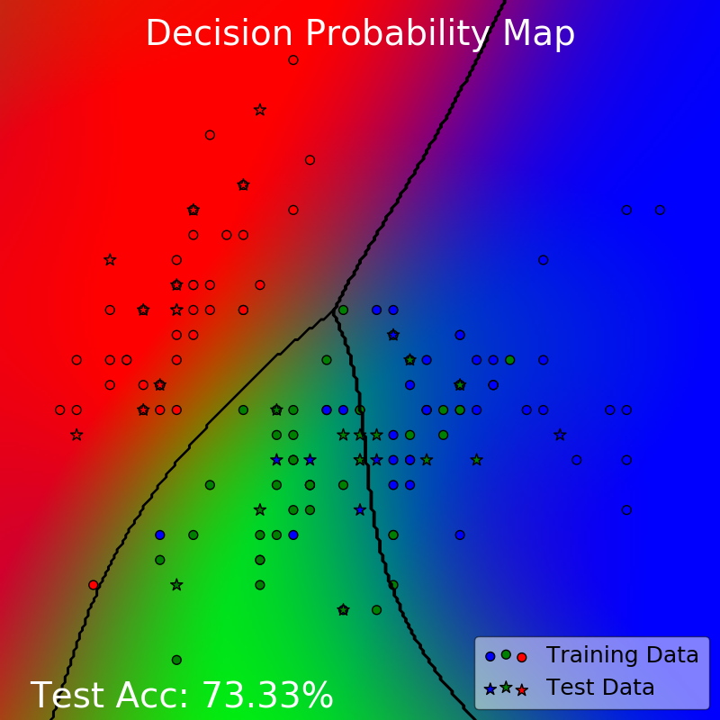
This is a perfectly reasonable model — simple and explains the data to a fairly decent degree at 73.33% test accuracy. In fact, due to the non-separable nature of the problem, this is the best test accuracy we could achieve here.

If we choose the wrong parameters, we may instead end up with models like below.

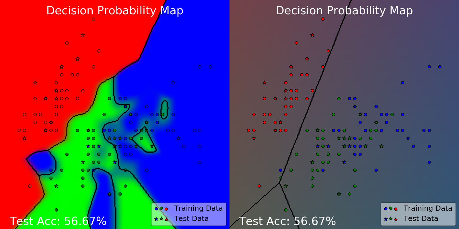
This is how much the model could change by changing its hyperparameters. Clearly, the one on the left has overfitted and the one on the right has underfitted. Both of them are sub-optimal with a test accuracy of 56.66%.

Now, I know what you are thinking. Isn’t underfitting and overfitting a standard problem in supervised learning? Don’t we have so many ways to deal with this already? For instance, cross validation would be the standard go-to approach for these kinds of problems.

Can’t we achieve good generlization like the first model with all those hyperparameter learning techniques that we already have?

Well, here is what happens when you employ current methods for learning hyperparameters of conditional mean embeddings.

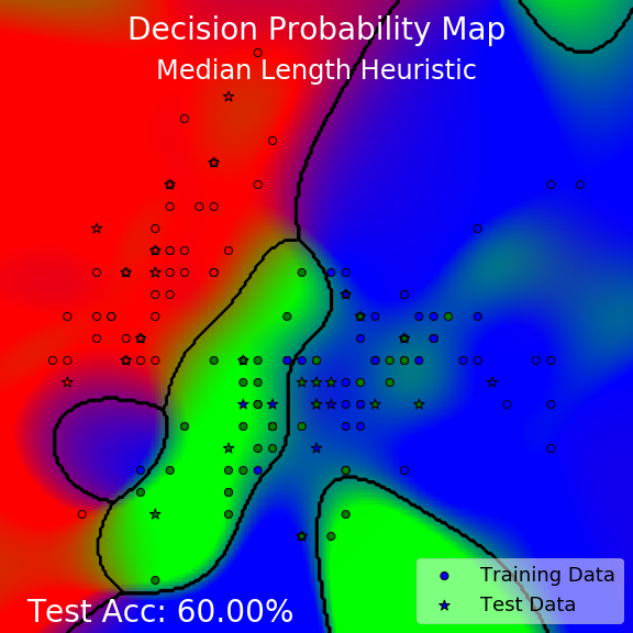
What?? They look kind of terrible!

Although, this should really come as no surprise for median length heuristic. It works by finding all the pairwise distances between all the data points, finding the median of those distances, and use that as a heuristic to set the length scale hyperparameter of the kernel. There are two problems with this. Firstly, not all hyperparameters are length scale hyperparameters! So, this technique is not generally applicable. Secondly, this heuristic does not make use of any target label information — it has no clue whether each point is a red, green, or blue dot, so it does not even leverage the essential information it needs to do a good job.

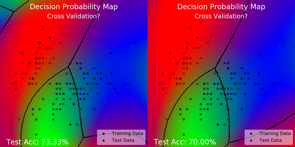
For cross validation, it actually did quite well, achieving at or close to the optimal test accuracy. However, despite the good test accuracy, would you say that the model has learned to generalize well? Pay attention to the corners, why are there unnatural patches of another color at those places? Can we really say that the model has learned a nice simple pattern to explain the data? Why is it doing this?

Well, we know how cross validation works — it works by minimizing the loss on some validation sets. Perhaps across many folds, but it has to be minimizing the loss on some data. We do not have any data at the corners we were complaining about, so of course cross validation is not going to address those areas. It never had information about those areas so whatever happens there is fair game.

You might think that we are being unfair to cross validation. After all, it still got a very decent test accuracy! We never had data at those corners to begin with, so who says that these patches are wrong? Perhaps if we actually collect data there, it does turn out to be a new color! So, it is not fair to measure its performance based on what it predicts in those areas.

However, I would argue that it should prefer to learn a simpler model as long as it is possible. This is a very simple toy example. Why shouldn’t our learning algorithm be capable of learning the nice simple pattern that generalizes well? We know that such a nice pattern is possible — we have just seen at the start of this section. So the problem is not the representational power of our model. The problem is rooted in our learning algorithm.

Furthermore, cross validation also has several problems. How many folds do we choose to use? What seed do we use and how should we randomize the splits? This is why I have shown two cases for cross validation with a question mark — the two are actually results from two different seeds, and produces slightly different results. Finally, having to train a model separately for each fold is also very expensive, especially if this is to happen every learning iteration.

The lesson here is that to ensure good generalization under limited data, it is not enough to just make sure our model performs well on validation sets. As we have limited data there are always places we lack information about where we still have to be able to make decent inference for.

What really needs to happen is that we need a sense of model complexity for the conditional mean embedding. We need to let the learning algorithm know that, in the face of seemingly equivalent models with similar validation performance, which ones would be a simpler explanation of the data that is more likely to be correct as per Occam’s razor.

This is one of the main contributions of our paper — a novel model complexity measure termed the Rademacher complexity bound that arises from learning theoretic bounds for the expected generalization risk.

Let us see how well our learning algorithm works on toy examples and verify that the Rademacher complexity bound (RCB) measures model complexity intuitively.

Three-Tailed Spiral

First up we have a sanity check. The spiral dataset is a simple but nonlinearly separable dataset with three classes. We begin with hyperparameters that result in an underfitted and oversimplified model with a test accuracy of 50%.

The goal here is two fold. Firstly, we want to see if our learning algorithm can learn patterns with the appropriate complexity to generalize well. Secondly, we want to see if our proposed Rademacher complexity bound (RCB) is interpretable as a model complexity measure.

This demonstration shows that our learning algorithm do learn hyperparameters that result in a model with appropriate complexity that generalizes well, driving test accuracy from 50% to at 99.33%. Critically, the RCB measure also aligns with our intuition that it should get higher as the model becomes more complex and curvy. Finally, the resulting model is a pleasing spiral pattern that one would expect for this dataset, instead of other crooked patterns that could still perform well on the test data but in an unnatural way.

Non-Separable Iris

Back to the non-separable iris scenario, we will begin with the initially overfitted and underfitted models shown before and apply our learning algorithm onto these two initial states.

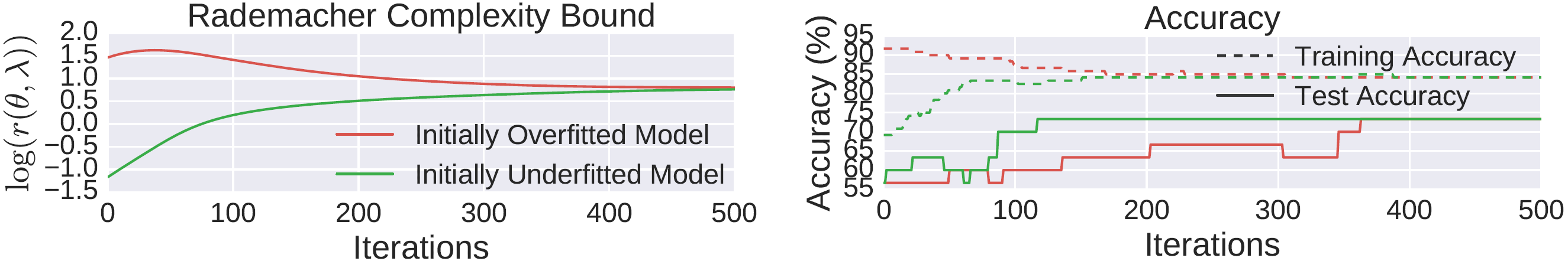
Amazingly, even though the model started from very different states, under our learning algorithm they converge to the same complexity balanced model — the one that we claimed was optimal for this data.

In particular, the RCB for the initially overfitted model starts off high and decreases over time, while the RCB for the initially underfitted model starts of low and increases over time. They both reach the same balanced complexity at the end of 500 iterations.

In terms of accuracy, even though the training accuracy for the initially overfitted model is decreasing, its test accuracy is improving throughout its learning. The learning algorithm knows to trade off performance on known data for the sake of a simpler model.

Our learning algorithm provides both an interpretable quantity, the Rademacher complexity bound, for model learning diagnostics, and a robust way to ensure good generalization in non-trivial scenarios.